Reduction in CUDA

August 24, 2025

Introduction

Reduction is an important mathematical operation in parallel computing. A reduction derives a single value from an array of values (like a sum, maximum, or average). It can be performed by sequentially going through every element of the array.

In this blog, we will look at different parallel reduction techniques in CUDA and compare the kernel execution times against PyTorch.

Kernel 1: Reduction Trees

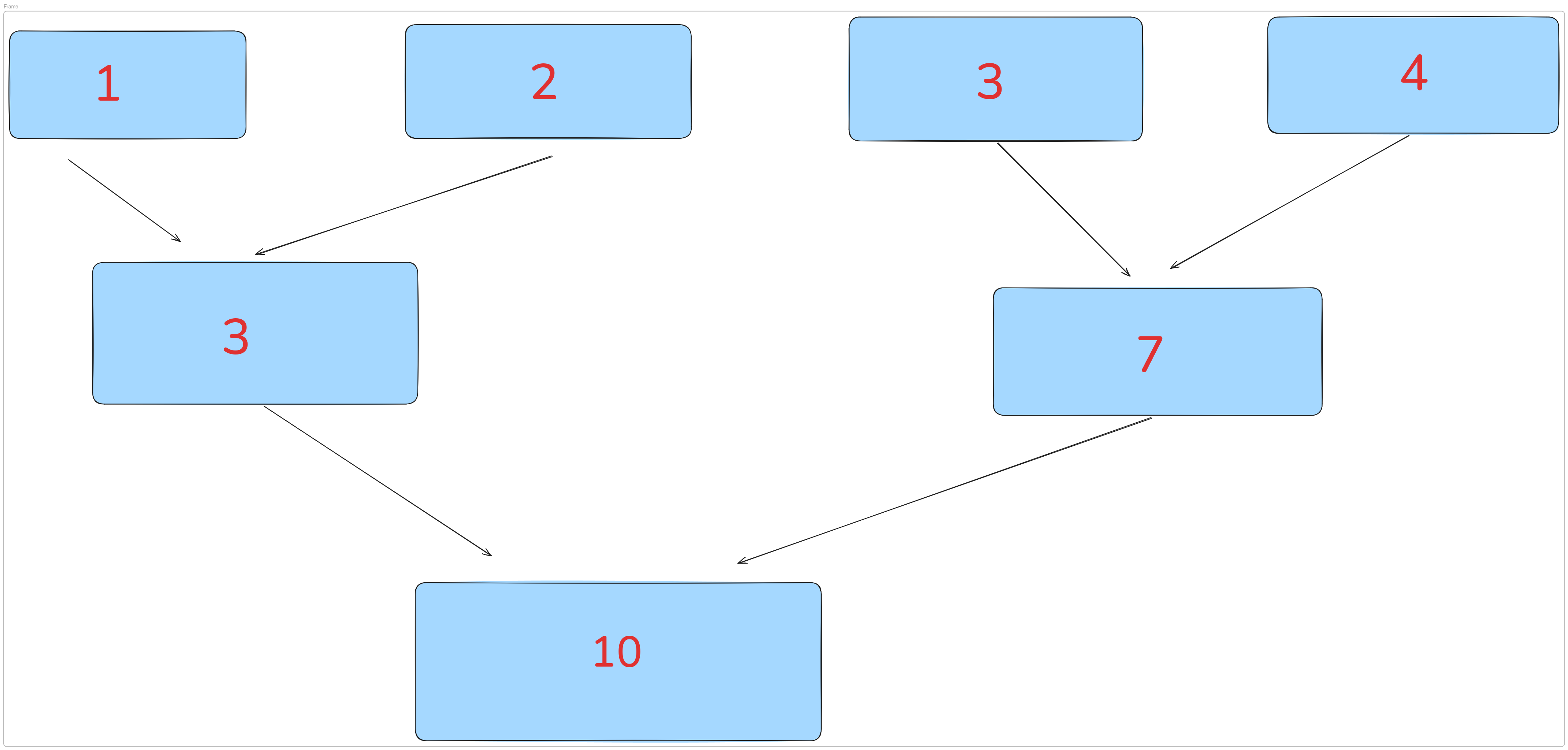
The parallel reduction tree is a very widely used technique for doing reduction. The basic concept is simple: take the sum of two consecutive, not yet summed elements, then keep doing this until all elements are combined into one. Since the additive (+) operation is associative, the basic intuition is:

sum = (a + b + c + d) = (a + b) + (c + d)

__global__ void reduce_naive(const float* g_idata, float* g_odata) {
    extern __shared__ float sdata[];

    unsigned int tid = threadIdx.x;
    unsigned int i = blockIdx.x * blockDim.x + threadIdx.x;

    sdata[tid] = g_idata[i];
    __syncthreads();

    // interleaved addressing - divergent branching + strided access
    for (unsigned int s = 1; s < blockDim.x; s *= 2) {
        if (tid % (2 * s) == 0) {
            sdata[tid] += sdata[tid + s];
        }
        __syncthreads();
    }

    if (tid == 0) g_odata[blockIdx.x] = sdata[0];
}

Kernel execution time: 118.324127 ms

The problem with this approach is that highly divergent code is very inefficient, and the % operator is quite slow. Here, only threads satisfying tid % (2 * s) == 0 are active in a warp. So a single warp ends up split between active and inactive threads. Since only half of the threads are active and half are inactive, it’s a waste of execution resources.

if (tid % (2 * s) == 0) {
    sdata[tid] += sdata[tid + s];
}

Kernel 2: Sequential Addressing

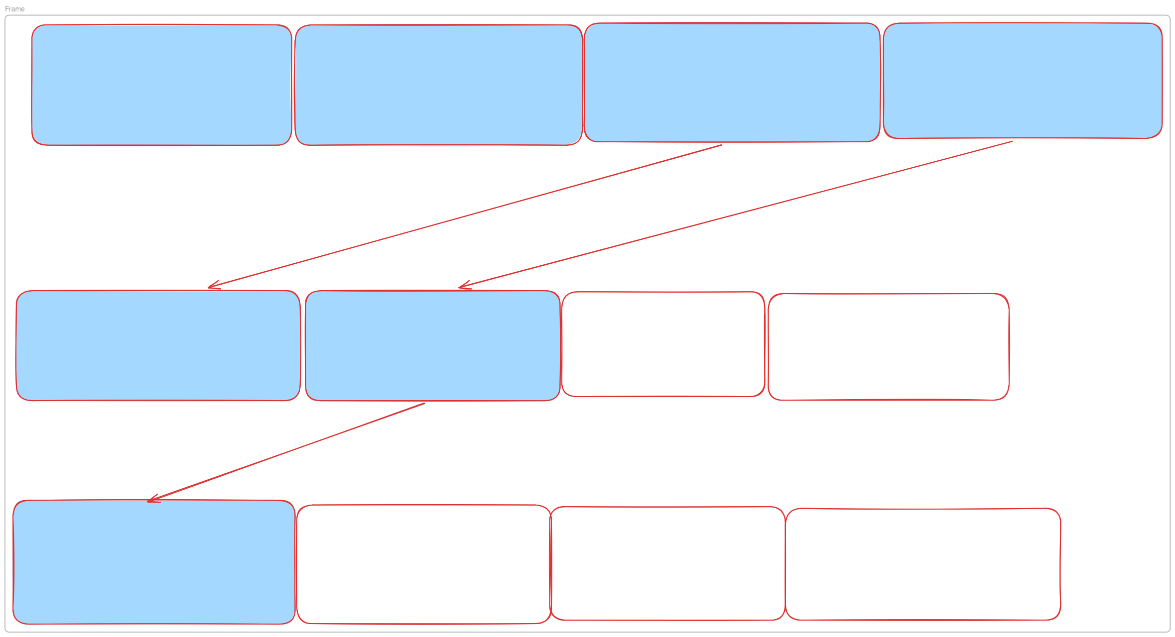
Sequential addressing solves the warp-divergence problem of Kernel 1. Now, within a warp (which consists of only 32 threads), either all threads are active or all are inactive. Fewer threads are also needed to execute the kernel. Here, we add the second half of the elements into the addresses of the first half, and keep doing this until all the elements are combined into one sum. So the basic intuition is:

sum = (a + b + c + d) = (a + c) + (b + d)

Imagine there are 512 elements and we run the reduction process. The first step will only take 256 threads and perform sums like sum[0] = sum[0] + sum[256], …, sum[255] = sum[255] + sum[511]. That’s how, at every step, the number of elements being reduced is halved, and so is the number of active threads halving both the element count and the thread count each step, until only 1 thread is left doing the final add.

__global__ void reduce_sequential(const float* g_idata, float* g_odata) {
    extern __shared__ float sdata[];

    unsigned int tid = threadIdx.x;
    unsigned int i = blockIdx.x * blockDim.x + threadIdx.x;

    sdata[tid] = g_idata[i];
    __syncthreads();

    // sequential addressing
    for (unsigned int s = blockDim.x / 2; s > 0; s >>= 1) {
        if (tid < s) {
            sdata[tid] += sdata[tid + s];
        }
        __syncthreads();
    }

    if (tid == 0) g_odata[blockIdx.x] = sdata[0];
}

Kernel execution time: 13.971296 ms -> roughly 8.5x faster than Kernel 1.

But the problem with this approach is that half of the threads are idle starting from the very first loop iteration. For reducing 512 elements, look at the very first iteration: s = blockDim.x / 2. Only threads with tid < s do any work that’s exactly half the threads in the block. The other half (tid >= s) just sit there doing nothing except waiting at __syncthreads().

Kernel 3: First Add During Load

We can further improve the kernel’s performance by combining the load from global memory with the first addition. Shared memory has much lower latency and higher bandwidth, so the idea is to load and add two elements from global memory into shared memory before starting the reduction work — this way, half of the threads aren’t left idle right away.

__global__ void reduce_first_add(const float* g_idata, float* g_odata) {
    extern __shared__ float sdata[];

    unsigned int tid = threadIdx.x;
    unsigned int i = blockIdx.x * (blockDim.x * 2) + threadIdx.x;

    sdata[tid] = g_idata[i] + g_idata[i + blockDim.x];
    __syncthreads();

    for (unsigned int s = blockDim.x / 2; s > 0; s >>= 1) {
        if (tid < s) {
            sdata[tid] += sdata[tid + s];
        }
        __syncthreads();
    }

    if (tid == 0) g_odata[blockIdx.x] = sdata[0];
}

Kernel execution time: 0.400064 ms -> a massive jump, about 35x faster than Kernel 2. Say blockDim.x = 512 (512 threads per block), and we’re using the “first add during load” scheme. Each block now covers blockDim.x * 2 = 1024 elements of the input array.

For block 0 specifically:

idx = blockIdx.x * (blockDim.x * 2) + tid
    = 0 * 1024 + tid
    = tid

So thread tid in block 0 reads g_idata[tid] and g_idata[tid + 512]:

tid = 0 ... sdata[0]   = g_idata[0]   + g_idata[0 + 512]
tid = 1 ... sdata[1]   = g_idata[1]   + g_idata[1 + 512]
tid = 2 ... sdata[2]   = g_idata[2]   + g_idata[2 + 512]
...
tid = 511 ... sdata[511] = g_idata[511] + g_idata[511 + 512]

Kernel 4: Unrolling the Last Warp

A warp only has 32 threads. Once a kernel’s reduction reaches the point where s <= 32, all the active threads belong to the same warp, and warps execute in lockstep (SIMT). This means we no longer need __syncthreads() calls, and we can unroll the remaining steps manually to avoid the loop overhead of if (tid < s) checks and unnecessary synchronization.

__global__ void reduce_unroll_last_warp(const float* g_idata, float* g_odata) {
    extern __shared__ float sdata[];

    unsigned int tid = threadIdx.x;
    unsigned int i = blockIdx.x * (blockDim.x * 2) + threadIdx.x;

    sdata[tid] = g_idata[i] + g_idata[i + blockDim.x];
    __syncthreads();

    // main loop now stops early, at s > 32
    for (unsigned int s = blockDim.x / 2; s > 32; s >>= 1) {
        if (tid < s) {
            sdata[tid] += sdata[tid + s];
        }
        __syncthreads();
    }

    // last warp - unrolled, no __syncthreads() needed
    if (tid < 32) {
        volatile float* smem = sdata;
        smem[tid] += smem[tid + 32];
        smem[tid] += smem[tid + 16];
        smem[tid] += smem[tid + 8];
        smem[tid] += smem[tid + 4];
        smem[tid] += smem[tid + 2];
        smem[tid] += smem[tid + 1];
    }

    if (tid == 0) g_odata[blockIdx.x] = sdata[0];
}

Kernel execution time: 0.304448 ms -> a smaller but still solid gain, about 1.3x faster than Kernel 3. Let’s visualize how this last-warp unrolling actually works and reduces the sum:

smem[tid] = smem[tid] + smem[tid + 32]

tid = 0 ... smem[0] = smem[0] + smem[32]
tid = 1 ... smem[1] = smem[1] + smem[33]
tid = 2 ... smem[2] = smem[2] + smem[34]

All 32 threads execute this on the same cycle. After this line, smem[0..31] holds 32 combined values.

smem[tid] = smem[tid] + smem[tid + 16]

tid = 0 ... smem[0] = smem[0] + smem[16]
          = old_smem[0] + old_smem[32] + old_smem[16] + old_smem[48]

smem[0] now holds the sum of 4 elements. After the next step, smem[0..15] holds 16 combined values from the original 64 elements.

Because all these threads belong to the same warp, we don’t need __syncthreads() here when one thread finishes an operation and moves to the next, the other threads in the warp finish that same operation in lockstep too. Every thread does its share of the work, and finally tid == 0 holds the sum of all 64 values:

smem[tid] += smem[tid + 32];  // 64 values -> 32 values
smem[tid] += smem[tid + 16];  // 32 values -> 16 values
smem[tid] += smem[tid + 8];   // 16 values -> 8 values
smem[tid] += smem[tid + 4];   // 8 values  -> 4 values
smem[tid] += smem[tid + 2];   // 4 values  -> 2 values
smem[tid] += smem[tid + 1];   // 2 values  -> 1 value

Kernel 5: Fully Optimized Kernel

template <unsigned int blockSize>
__global__ void reduce_final(const float* g_idata, float* g_odata, unsigned int n) {
    extern __shared__ float sdata[];

    unsigned int tid = threadIdx.x;
    unsigned int i = blockIdx.x * (blockSize * 2) + tid;
    unsigned int gridSize = blockSize * 2 * gridDim.x;

    sdata[tid] = 0.0f;
    while (i < n) {
        sdata[tid] += g_idata[i] + g_idata[i + blockSize];
        i += gridSize;
    }
    __syncthreads();

    if (blockSize >= 1024) { if (tid < 512) { sdata[tid] += sdata[tid + 512]; } __syncthreads(); }
    if (blockSize >= 512)  { if (tid < 256) { sdata[tid] += sdata[tid + 256]; } __syncthreads(); }
    if (blockSize >= 256)  { if (tid < 128) { sdata[tid] += sdata[tid + 128]; } __syncthreads(); }
    if (blockSize >= 128)  { if (tid < 64)  { sdata[tid] += sdata[tid + 64];  } __syncthreads(); }

    if (tid < 32) {
        volatile float* smem = sdata;
        if (blockSize >= 64) smem[tid] += smem[tid + 32];
        if (blockSize >= 32) smem[tid] += smem[tid + 16];
        if (blockSize >= 16) smem[tid] += smem[tid + 8];
        if (blockSize >= 8)  smem[tid] += smem[tid + 4];
        if (blockSize >= 4)  smem[tid] += smem[tid + 2];
        if (blockSize >= 2)  smem[tid] += smem[tid + 1];
    }

    if (tid == 0) g_odata[blockIdx.x] = sdata[0];
}

Kernel execution time: 0.245120 ms -> the fastest of the five, about 1.24x faster than Kernel 4, thanks to the grid-stride loop letting fewer blocks do more work per thread.

This is the final, fully optimized kernel. It uses a grid-stride loop so that each thread accumulates values from multiple locations across the entire array before any shared memory reduction even begins.

Benchmarking

I benchmarked all five kernels against PyTorch’s sum() and saw a clear, consistent improvement from Kernel 1 through Kernel 5. Compared to PyTorch, though, we’re still not at the same level, kept intentionally simple since I’m still learning this material. PyTorch is faster because it leans on more advanced techniques.

Setup: N = 4,194,304 elements

warm-up runs = 10

timed runs (averaged) = 50

Kernel	Result	Avg time (ms)	Speedup vs K1	Speedup vs PyTorch
Kernel 1: Naive (interleaved addressing)	4,194,304.0000	1.06026	1.00x	0.08x
Kernel 2: Sequential addressing	4,194,304.0000	0.62353	1.70x	0.14x
Kernel 3: First add during load	4,194,304.0000	0.33532	3.16x	0.27x
Kernel 4: + unroll last warp	4,194,304.0000	0.21686	4.89x	0.41x
Kernel 5: Final (grid-stride + unrolled)	4,194,304.0000	0.14012	7.57x	0.64x
PyTorch sum()	4,194,304.0000	0.08934	11.87x	1.00x

Expected result: 4,194,304.0000 -> every kernel matches PyTorch’s output exactly, so correctness is confirmed across all five implementations.

A more detailed, per stage profile (GPU memory allocation, host-to-device transfer, kernel execution, device-to-host transfer) shows where the real cost sits and how it shifts as the kernels improve:

Kernel	GPU allocation (ms)	Host → Device (ms)	Kernel execution (ms)	Device → Host (ms)
Kernel 1: Naive	0.274560	8.063296	118.324127	0.064480
Kernel 2: Sequential addressing	0.193120	3.846208	13.971296	0.038496
Kernel 3: First add during load	0.206976	3.891072	0.400064	0.022304
Kernel 4: + unroll last warp	0.196672	3.860352	0.304448	0.025664
Kernel 5: Final (grid-stride + unrolled)	0.194496	3.782880	0.245120	0.049280

References

• Optimizing Parallel Reduction in CUDA (NVIDIA/Uni Graz lecture notes)
• Lei Mao — CUDA Reduction
• CUDA MODE Notes — Lecture 9

While writing this blog, I did my best to avoid mistakes, but a few issues may still pop up. If you spot any errors, please email me at saikatsingha0q@gmail.com. Thanks for reading!